
| Home| Contens | |
Description of technique
Instant point source can be described by the moment tensor - a
symmetric
3x3 matrix ![]() .
Seismic moment
.
Seismic moment ![]() is defined by equation
is defined by equation ![]() ,
where
,
where ![]() is transposed moment tensor
is transposed moment tensor ![]() ,
and
,
and 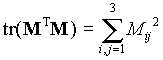 .
Moment tensor of any event can be presented in the form
.
Moment tensor of any event can be presented in the form ![]() ,
where matrix
,
where matrix ![]() is normalised by condition
is normalised by condition ![]() .
.
We are considering a double couple instant point source (a pure
tangential
dislocation) at a depth h. Such a source can be given by 5 parameters:
double couple depth, its focal mechanism which is characterising by
three
angles: strike, dip and slip or by two unit vectors (direction of
principal
tension T and direction of principal compression P) and seismic
moment ![]() .
Four of these parameters we determine by a systematic exploration of
the
four dimensional parametric space, and the 5-th parameter
.
Four of these parameters we determine by a systematic exploration of
the
four dimensional parametric space, and the 5-th parameter ![]() - solving the problem of minimisation of the misfit between observed
and
calculated surface wave amplitude spectra for every current combination
of all other parameters.
- solving the problem of minimisation of the misfit between observed
and
calculated surface wave amplitude spectra for every current combination
of all other parameters.
Under assumptions mentioned above the relation between the spectrum
of the displacements ![]() in any surface wave and the total moment tensor
in any surface wave and the total moment tensor ![]() can be expressed by following formula
can be expressed by following formula
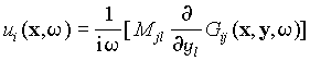 (1)
(1)
i,j = 1,2,3 and the summation convention for repeated subscripts is
used. ![]() in equation (1) is the spectrum of Green function for the chosen model
of medium and wave type (see Levshin, 1985; Bukchin, 1990),
in equation (1) is the spectrum of Green function for the chosen model
of medium and wave type (see Levshin, 1985; Bukchin, 1990), ![]() -
source location. We assume that the paths from the earthquake source to
seismic stations are relatively simple and are well approximated by
weak
laterally inhomogeneous model (Woodhouse, 1974; Babich et al., 1976).
The
surface wave Green function in this approximation is determined by the
near source and near receiver velocity structure, by the mean phase
velocity
of wave, and by geometrical spreading. The amplitude spectrum |
-
source location. We assume that the paths from the earthquake source to
seismic stations are relatively simple and are well approximated by
weak
laterally inhomogeneous model (Woodhouse, 1974; Babich et al., 1976).
The
surface wave Green function in this approximation is determined by the
near source and near receiver velocity structure, by the mean phase
velocity
of wave, and by geometrical spreading. The amplitude spectrum |![]() |
defined by formula (1) does not depend on the average phase velocity of
the wave. In such a model the errors in source location do not affect
the
amplitude spectrum (Bukchin, 1990). The average phase velocities of
surface
waves are usually not well known. For this reason as a rule we use only
amplitude spectra of surface waves for determining source parameters
under
consideration. We use observed surface wave phase spectra only for very
long periods.
|
defined by formula (1) does not depend on the average phase velocity of
the wave. In such a model the errors in source location do not affect
the
amplitude spectrum (Bukchin, 1990). The average phase velocities of
surface
waves are usually not well known. For this reason as a rule we use only
amplitude spectra of surface waves for determining source parameters
under
consideration. We use observed surface wave phase spectra only for very
long periods.
Surface wave amplitude spectra inversion
If all characteristics of the medium are known the representation
(1)
gives us a system of equations for parameters defined above. Let us
consider
now a grid in the space of these 4 parameters. Let the models of the
media
be given. Using formula (1) we can calculate the amplitude spectra of
surface
waves at the points of observation for every possible combination of
values
of the varying parameters. Comparison of calculated and observed
amplitude
spectra give us a residual ![]() for
every point of observation, every wave and every frequency
for
every point of observation, every wave and every frequency ![]() .
Let
.
Let ![]() be any observed value of the spectrum, i = 1,?,N;
be any observed value of the spectrum, i = 1,?,N; ![]() -
corresponding residual of |
-
corresponding residual of |![]() |.
We define the normalised amplitude residual by formula
|.
We define the normalised amplitude residual by formula
 .
(2)
.
(2)
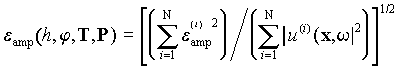
The optimal values of the parameters that minimize eamp
we consider as estimates of these parameters. We search them by a
systematic
exploration of the five dimensional parameter space. To characterize
the
degree of resolution of every of these source characteristics we
calculate
partial residual functions. Fixing the value of one of varying
parameters
we put in correspondence to it a minimal value of the residual eamp on
the set of all possible values of the other parameters. In this way we
define one residual function on scalar argument and two residual
functions
on vector argument corresponding to the scalar and two vector varying
parameters: ![]() ,
, ![]() and
and ![]() .
The value of the parameter for which the corresponding function of the
residual attains its minimum we define as estimate of this parameter.
At
the same time these functions characterize the degree of resolution of
the corresponding parameters. From geometrical point of view these
functions
describe the lower boundaries of projections of the 4-D surface of
functional
.
The value of the parameter for which the corresponding function of the
residual attains its minimum we define as estimate of this parameter.
At
the same time these functions characterize the degree of resolution of
the corresponding parameters. From geometrical point of view these
functions
describe the lower boundaries of projections of the 4-D surface of
functional ![]() on
the coordinate planes.
on
the coordinate planes.
It is well known that the focal mechanism can not be uniquely determined from surface wave amplitude spectra. There are four different focal mechanisms which will radiate this same surface wave amplitude spectra. These four equivalent solutions represent two pairs of mechanisms symmetric with respect to the vertical axis, and within the pair differ from each other by the opposite direction of slip.
To get a unique solution for the focal mechanism we have to use in
the
inversion additional observations. For these purpose we use very long
period
phase spectra of surface waves or polarities of P wave first arrivals.
Joint inversion of surface wave amplitude and phase spectra
Using formula (1) we can calculate for chosen frequency range the
phase
spectra of surface waves at the points of observation for every
possible
combination of values of the varying parameters. Comparison of
calculated
and observed phase spectra give us a residual ![]() for
every point of observation, every wave and every frequency
for
every point of observation, every wave and every frequency ![]() .
We define the normalised amplitude residual by formula
.
We define the normalised amplitude residual by formula
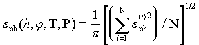 .
(3)
.
(3)
We determine the joint residual ![]() by
formula
by
formula
![]() .
(4)
.
(4)
Joint inversion of surface wave amplitude spectra and P wave polarities
Calculating radiation pattern of P waves for every current
combination
of parameters we compare it with observed polarities. The misfit
obtained
from this comparison we use to calculate a joint residual of surface
wave
amplitude spectra and polarities of P wave first arrivals. Let ![]() be
the residual of surface wave amplitude spectra,
be
the residual of surface wave amplitude spectra, ![]() -
the residual of P wave first arrival polarities (the number of wrong
polarities
divided by the full number of observed polarities), then we determine
the
joint residual
-
the residual of P wave first arrival polarities (the number of wrong
polarities
divided by the full number of observed polarities), then we determine
the
joint residual ![]() by
formula
by
formula
![]() .
(5)
.
(5)
Before inversion we apply to observed polarities a smoothing
procedure
which we will describe here briefly.
Let us consider a group of observed polarities (+1 for compression
and -1 for dilatation) radiated in directions deviating from any medium
one by a small angle. This group is presented in the inversion
procedure
by one polarity prescribing to this medium direction. If the number of
one of two types of polarities from this group is significantly larger
then the number of opposite polarities, then we prescribe this polarity
to this medium direction. If no one of two polarity types can be
considered
as preferable, then all these polarities will not be used in the
inversion.
To make a decision for any group of n observed polarities we calculate
the sum ![]() ,
where n+ is the number of compressions and
,
where n+ is the number of compressions and ![]() is the number of dilatations. We consider one of polarity types as
preferable
if |m| is larger then its standard deviation in the case when +1 and -1
appear randomly with this same probability 0.5. In this case n+ is a
random
value distributed following the binomial low. For its average we
have
is the number of dilatations. We consider one of polarity types as
preferable
if |m| is larger then its standard deviation in the case when +1 and -1
appear randomly with this same probability 0.5. In this case n+ is a
random
value distributed following the binomial low. For its average we
have ![]() ,
and for dispersion
,
and for dispersion ![]() .
Random value m is a linear function of n+ such that
.
Random value m is a linear function of n+ such that ![]() .
So following equations are valid for the average, for the dispersion,
and
for the standard deviation s of value m
.
So following equations are valid for the average, for the dispersion,
and
for the standard deviation s of value m
![]() ,
, ![]() ,
and
,
and![]() .
.
As a result, if the inequality ![]() is valid then we prescribe +1 to the medium direction if
is valid then we prescribe +1 to the medium direction if ![]() ,
and -1 if
,
and -1 if ![]() .
.
References
V.M. Babich, B.A. Chikachev and T.B. Yanovskaya, 1976. Surface waves in a vertically inhomogeneous elastic half-space with weak horizontal inhomogeneity, Izv. Akad. Nauk SSSR, Fizika Zemli, 4, 24-31.
B.G. Bukchin, 1990. Determination of source parameters from surface waves recordings allowing for uncertainties in the properties of the medium, Izv. Akad. Nauk SSSR, Fizika Zemli, 25, 723-728.
A.V. Lander, 1989. Frequency-time analysis. In: V.I. Keilis-Borok (Editor), Seismic surface waves in a laterally inhomogeneous earth. Kluwer Academic Publishers Dordrecht, 153-163.
A.L. Levshin, 1985. Effects of lateral inhomogeneity on surface wave amplitude measurements, Annles Geophysicae, 3, 4, 511-518.
J.H. Woodhouse, 1974. Surface waves in the laterally varying
structure.
Geophys.
J. R. astr. Soc., 90, 12, 713-728.