for
Data base creation
Frequency-time analysis
Moment Tensor & Source Depth Inversion
Any distribution scheme
of our package provides corresponding
example. Every example contains complete set of input data and output
results.
Data base creation
Frequency-time analysis
Moment Tensor & Source Depth Inversion
Example Directory structure:
Root examples directory: /opt/fmt/example.
/opt/fmt/example/Seed2Db/ - Creating Data base.
/opt/fmt/example/Ftan/ - Frequency-time analysis program.
/opt/fmt/example/MomTens/ - Moment Tensor & Source Depth Inversion Program.
I Creating Data base
1.1 Enter directory /opt/fmt/example/Seed2Db
Subdirectories:
SeedVols/ - the directory for the input seed volumes which contains just one seed volume: colima.seed
Dbase/ - the directory for the output resulting dbase
work/ - the directory for the working materials.
All of these directories must be created in advance!
1.2 Execute command Fmt4Db
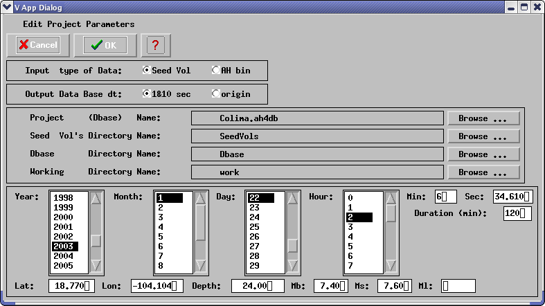
1.3. Use the icon and fill the empty boxes, lists, radio buttons.
1.3..1 Input type of Data: Click button "Seed Vol" - Dbase will be created from seed volumes
1.3..2 Output Data Base dt: Click button "1&10 sec" - Input time series will be decimated to 1&10 seconds.
1.3..3 Duration (min): Type "120" - The duration of each resulting Dbase record will not exceed 120 minutes.
1.3..4 Project (Dbase) Name: - Push “browse” button to choose "Seed2Db" and type"Colima" as project name. This name will become a root name of resulting dbase. The program will add to the project name fixed extension “ah4db”. The project name will be "Colima.ah4db" and Dbase Root Name will be "Colima".
1.3..5 Seed Vol's Directory Name: - Browse directory "Seed2Db" and click on "SeedVols" directory which contains seed volume. The name of this directory will appear in browser’s “Selection” box . Click "OK" button and "SeedVols" will appear in the boxSeed Vol's Directory Name .
1.3..6 Dbase Directory Name: - Browse directory "Seed2Db" and click on "Dbase" directory which will contain the output dbase.
Working Directory Name: - Browse directory "Seed2Db" and click on "work" directory which will be used for working materials.
1.3..7 Fill the rest boxes and lists as it is shown bellow.
Subdirectories:
SeedVols/ - the directory for the input seed volumes which contains just one seed volume: colima.seed
Dbase/ - the directory for the output resulting dbase
work/ - the directory for the working materials.
All of these directories must be created in advance!
1.2 Execute command Fmt4Db
1.3. Use the icon
1.3..1 Input type of Data: Click button "Seed Vol" - Dbase will be created from seed volumes
1.3..2 Output Data Base dt: Click button "1&10 sec" - Input time series will be decimated to 1&10 seconds.
1.3..3 Duration (min): Type "120" - The duration of each resulting Dbase record will not exceed 120 minutes.
1.3..4 Project (Dbase) Name: - Push “browse” button to choose "Seed2Db" and type"Colima" as project name. This name will become a root name of resulting dbase. The program will add to the project name fixed extension “ah4db”. The project name will be "Colima.ah4db" and Dbase Root Name will be "Colima".
1.3..5 Seed Vol's Directory Name: - Browse directory "Seed2Db" and click on "SeedVols" directory which contains seed volume. The name of this directory will appear in browser’s “Selection” box . Click "OK" button and "SeedVols" will appear in the boxSeed Vol's Directory Name .
1.3..6 Dbase Directory Name: - Browse directory "Seed2Db" and click on "Dbase" directory which will contain the output dbase.
Working Directory Name: - Browse directory "Seed2Db" and click on "work" directory which will be used for working materials.
1.3..7 Fill the rest boxes and lists as it is shown bellow.
Push button “OK”.
1.3..8 Push button to save all information
into "Colima.ah4db" project file name for future using.
to save all information
into "Colima.ah4db" project file name for future using.
1.4. Push the button .
.
These lists allow user to choose suitable station for transmission to Dbase using buttons: ,
, ,
, ,
,
For the confirmation of changes close this windows using button “OK”.
1.5. Push the button and wait.
1.3..8 Push button
1.4. Push the button
These lists allow user to choose suitable station for transmission to Dbase using buttons:
For the confirmation of changes close this windows using button “OK”.
1.5. Push the button
II. Floating filtering of Colima earthquake records
2.1. Enter directory /opt/fmt/example/Ftan2.2. Execute command:
ftan
2.3. New/Open start window will appear.
Click on New tab
Brows:
/opt/fmt/example/Seed2Db/Dbase/Colima_l.wfdisc
/opt/fmt/example/Seed2Db/Dbase/Colima.instrument
/opt/fmt/example/Seed2Db/Dbase/Colima origin
Click on OK. Start window will disappear.
2.4. Click button
short period zero = 80, short period corner = 90, long period corner = 260, long period zero = 280.
2.5. Click button
group velocity from 2.5 to 6, periods from 80 to 280.
2.6. Until you didn’t select a station and a channel to be processed the light of semaphore button is red
2.7. To apply bandpass filtering click on the button
2.8. Click on the button
2.9. To save results click the button
Click component toggle buttons required to be saved. Click OK button to save records.
2.10. Select next station-channel. Button
2.11. After you finished the processing of all Colima records push the button
Recommended components to be saved and correspondent period ranges for floating filtering:
Record Tmin Tmax
AAK.LHT 100.00 200.00
AAK.LHZ 100.00 250.00
CTAO.LHT 150.00 250.00
CTAO.LHZ 150.00 250.00
KONO.LHZ 110.00 250.00
LVC.LHZ 120.00 200.00
MTE.LHT 105.00 200.00
MTE.LHZ 105.00 250.00
NNA.LHT 100.00 250.00
PTCN.LHZ 100.00 200.00
RCBR.LHT 115.00 200.00
RCBR.LHZ 130.00 220.00
RPN.LHT 140.00 250.00
RPN.LHZ 110.00 250.00
SNAA.LHT 100.00 200.00
SNAA.LHZ 100.00 250.00
TAU.LHT 130.00 250.00
TAU.LHZ 130.00 250.00
WAKE.LHT 110.00 200.00
WAKE.LHZ 110.00 250.00
YAK.LHT 110.00 250.00
YAK.LHZ 115.00 250.00
YSS.LHT 110.00 200.00
<>YSS.LHZ 130.00 250.00
<>
<>
<>
III. Moment Tensor & Source
Depth Inversion for Colima earthquake
3.1. Enter
directory /opt/fmt/example/MomTens.
3.2. Execute command
MomTens
The main window of the program will appear.
3.3. Push button
Define Project Directory - type Project Name (T100-250);
Filtered Wave Form Disc DB Name - browse directory /opt/fmt/example/Ftan/FLT , and click table.wfdisc.
Instrument, Site, Sensor DB Root Names - browse directory /opt/fmt/example/Seed2Db/Dbase/Colima.instrument
and click ‘Colima.site’
Origin Info Event Db Name - browse directory /opt/fmt/example/Seed2Db/Dbase/Dbase
and click ‘Colima.origin’
Note: Next time you can just use
3.4. To select records to be used for the inversion push button
3.5. Push button
Click on the button ‘3SMAC MODEL’ – the structure models for all stations will be calculated. Click on the model 000, and after on the radio button ‘Get Source Model from Model List’. Click ‘OK’.
3.6. Push button
We recommend following spectral bands to be used in the inversion
(Spectral Range for every wave):
Record Tmin Tmax
AAK.LHT 100.00 200.00
AAK.LHZ 100.00 250.00
CTAO.LHT 150.00 250.00
CTAO.LHZ 150.00 250.00
KONO.LHZ 110.00 250.00
LVC.LHZ 120.00 200.00
MTE.LHT 105.00 200.00
MTE.LHZ 105.00 250.00
NNA.LHT 100.00 250.00
PTCN.LHZ 100.00 200.00
RCBR.LHT 115.00 200.00
RCBR.LHZ 130.00 220.00
RPN.LHT 140.00 250.00
RPN.LHZ 110.00 250.00
SNAA.LHT 100.00 200.00
SNAA.LHZ 100.00 250.00
TAU.LHT 130.00 250.00
TAU.LHZ 130.00 250.00
WAKE.LHT 110.00 200.00
WAKE.LHZ 110.00 250.00
YAK.LHT 110.00 250.00
YAK.LHZ 115.00 250.00
YSS.LHT 110.00 200.00
YSS.LHZ 130.00 250.00
Parameters to be given in the right frame (Spectral rage):
Tmin=100, Tmax=250, Nw=18, N points FFT = 32768
Type in the text box at the bottom 150.
Push 'Get' button.
3.7. Push button
Recomended grid characteristics:
0.0 - Initial Depth
5.0 - Depth Step
11 - Number of Depth Values
15.0 - Initial Dip
15.0 - Dip Step
6 - Number of Dip Values
0.0 - Initial Strike
15.0 - Strike Step
12 - Number of Strike Values
0.0 - Initial Slip
15.0 - Slip Step
12 - Number of Slip Values
3.8. Push the button
Push the arrow in the combo box, choose the angle of polarity data smoothing (10 degrees), Push radio button ‘bulletin’. Push radio button ‘manually’, and print in edit box at the bottom ‘7.2’- the value of P-wave velocity in the source location. Confirm by pushing OK.
3.9. Push the button
3.10. View of results:
General
| Copyright © 1998 - 2005 Mitpan | Fmt-1.40 |